Simulation
Simulation is an important step to check that models produce expected patterns of behaviour. The process involves taking a series of task stimuli and feeding them into a learning model and observation model with a given set of parameter values to produce behaviour predicted by these particular parameter values.
To facilitate this process, the DMModel class has a simulate method, that provides the ability to simulate behaviour for a given model across parameter values, and produces outputs necessary to evaluate the simulated behaviour.
At a basic level, the simulate method can be called with a series of outcomes (e.g. reward/no reward for a given stimulus) as a .txt file or a numpy array, along with dictionaries of parameter values for the learning and observation models. For example:
model.simulate(outcomes, learning_parameters={'value': 0.5, 'alpha':0.3},
               observation_parameters={'b':3})
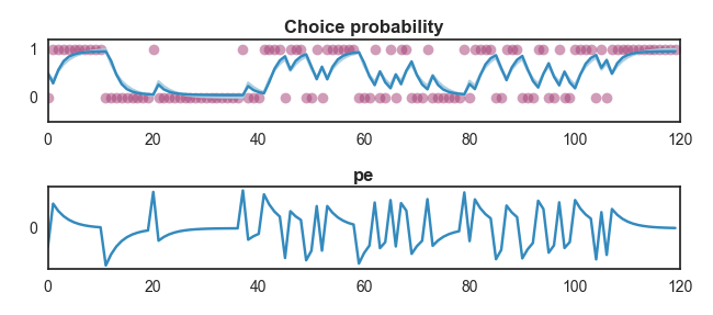
This will simulate behaviour according to the model’s responses to the given outcomes at the provided parameter values. By “behaviour” here we refer to the probability of choosing a given action. The simulate method will also produce plots of the simulated probability, along with any other variables provided by the learning and observation models (such as prediction errors or any other values returned by the model functions).
It can be useful to save the output of a simulation run to a file in the same format as real subjects’ data, and it is possible to do this by providing a value for the response_file argument of the simulate method. This will simulate choices on each trial based on the calculated probability of choosing a given action, and write these to a response file, along with subject IDs (subjects are named after the model parameters used to simulate them) and columns listing the provided parameter values for the simulation.
model.simulate(outcomes, learning_parameters={'value': 0.5, 'alpha':0.3},
               observation_parameters={'b':3}, response_file='simulated_data.csv')
It is also possible to simulate multiple subjects by providing a value for the n_subjects argument of the simulate method. This will generate additional sets of randomly determined choice data for each subject. Note that this only has an effect if there is some degree of randomness in the simulated data, for example when simulating binary choices from estimated choice probabilities.
Results of the most recent simulation are saved in the simulated attribute of the model instance. This takes the format of a dictionary containing the parameters values provided to the learning model, those provided to the observation model, and the results of the simulation. The simulation results take the form of a dictionary with entries representing the name of every variable returned by the model (e.g. estimated value, action probability, prediction errors etc.) and their value. This makes it relatively simple to access results from a range of simulations. For example, to retrieve the prediction errors given by the most recent simulation, we can use the following code.
>>> prediction_errors = model_rw.simulated['sim_results']['pe']
>>> print prediction_errors[:10]
[-0.5  0.65  0.455  0.3185  0.22295  0.156065  0.1092455  0.07647185  0.0535303  0.03747121]
The position of the values returned by the simulate method relative to each trial is important to be aware of, and differs depending on the type of variable being returned. The estimated value, and any other variable that is entered into the learning model’s calculation at each step is provided prior to the model seeing the outcome of the trial. For instance, if we set the initial estimated value at 0.5, the estimated value in the first trial of the simulated data will be 0.5. In contrast, other outputs (such as prediction errors) are provided on the same trial as the outcome. So for example the first prediction error would be the prediction error produced by the first trial.
If multiple subjects are simulated, the arrays for each variable returned by the simulation become two-dimensional (n_trials, n_subjects).
>>> prediction_errors_multisubject = model_rw.simulated['sim_results']['pe']
>>> print prediction_errors_multisubject.shape
(120L, 3L)
It is also possible to simulate multiple runs per subject by using the runs_per_subject argument. If an integer is given, a “Run” column will be produced in the response file, and each run for the subject will use the same parameter values. Note that this process is essentially identical to simulating multiple subjects except for the labelling in the output file (i.e. being labelled as a run instead of a subject) - this simply makes it simpler when fitting models to simulated data that involve multiple runs.
It is possible to simulate data from multiple values of a given parameter by simply entering the parameter values as a list rather than a single value. If each parameter has an equal number of values and the combinations argument is set to false, each simulation will represent a position in the lists of parameters. For example, if given the learning parameters {'a' : [0, 1], 'b': [0.1, 0.2], the simulation will generate one set of simulated data where a is set to 0 and b is set to 0.1, and another set of data where a is 1 and b is 0.2.
If the combinations argument is set to true, data will be simulated from every combination of the parameters provided. In the above example, this would lead to 4 simulations (0 & 0.1, 0 & 0.2, 1 & 0.1, 1 & 0.2).
The outcomes provided to the simulate method can take the form of an array with different outcomes for each subject (i.e. an array of the shape n_trials, n_subjects), or if a one-dimensional outcome array is provided this will be used for each combination of parameter values.
Simulations can also be run using a dataframe.
Parameter recovery
Parameter recovery tests the ability to determine parameter values from observed behavioural data simulated with known parameter values. For example, if we simulated behaviour using a Rescorla-Wagner learning model with an alpha value of 3, our model fitting procedures should return an alpha value of 3 when we attempt to fit a Rescorla-Wagner model to this data. DMpy provides a couple of functions to assist with this process. Firstly, when data is simulated using the DMModel class simulate method and saved to a csv file, the generated response file will include columns containing the values of each parameter used to simulate the data.
If a response file including these columns is fed into any of the DMModel class’s fit methods, it will automatically include these values in its output table for each subject and estimate Pearson correlations between the true and recovered parameter values (saved in the .recovery_correlations attribute of the model), along with producing plots to illustrate these.
In order for this to work properly, it’s advisable to simulate across a range of parameter values. This is simple to do by providing lists of values in the parameter dictionary rather than single values. If multiple values are provided for more than one parameter, all possible combinations of these parameter values will be simulated. Be aware that if many parameter values are provided, this can rapidly lead to a very large number of simulated datasets and cause problems!
This is an example of parameter recovery with a Rescorla-Wagner model, where we’re assessing our ability to recover the alpha parameter. To simulate across a range of values of alpha, we provide a range from 0.1 to 0.9 in steps of 0.1 using np.arange(0.1, 1, 0.1).
>>> sim_rw = model_rw.simulate(outcomes, n_subjects=50,
>>>                            response_file='parameter_recovery.csv',
>>>                            learning_parameters={'value': 0.5, 'alpha0': np.arange(0.1, 1, 0.1)},
>>>                            observation_parameters={'b':3})
Finished simulating
Saving simulated responses to parameter_recovery.csv
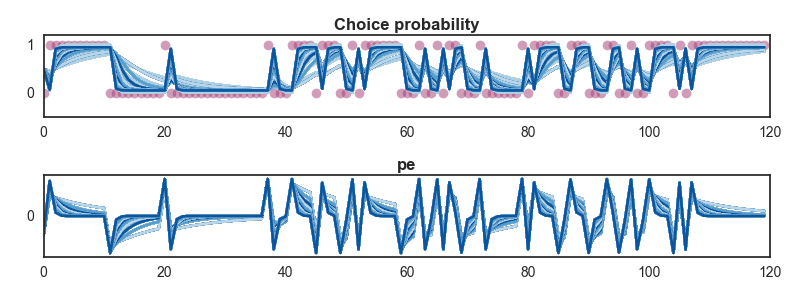
The simulation plots also now plot estimated probabilities and other values across the range of parameter values provided.
If we now fit our model to this data, we can see whether the alpha parameter is recovered successfully.
>>> model_rw.fit_MAP(outcomes, sim_rw)
Loading data
Loading multi-subject data with 450 subjects
Loaded data, 450 subjects with 120 trials
|
-------------------Finding MAP estimate-------------------
|
Performing model fitting for 450 subjects
|
Optimization terminated successfully.
 Current function value: 21874.952537
 Iterations: 45
 Function evaluations: 72
 Gradient evaluations: 72
|
 Performing parameter recovery tests...
           alpha0                   Subject  alpha0_sim  value_sim
    0    0.172732    alpha0.0.1.value.0.5_0         0.1        0.5
    1    0.129099    alpha0.0.1.value.0.5_1         0.1        0.5
    2    0.146754   alpha0.0.1.value.0.5_10         0.1        0.5
    3    0.111058   alpha0.0.1.value.0.5_11         0.1        0.5
    4    0.127479   alpha0.0.1.value.0.5_12         0.1        0.5
|
Finished model fitting in 30.8701867692 seconds
The parameter table has our simulated values in addition to the estimated values for each subject, and these are saved in the model’s .parameter_table attribute.
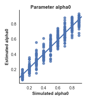
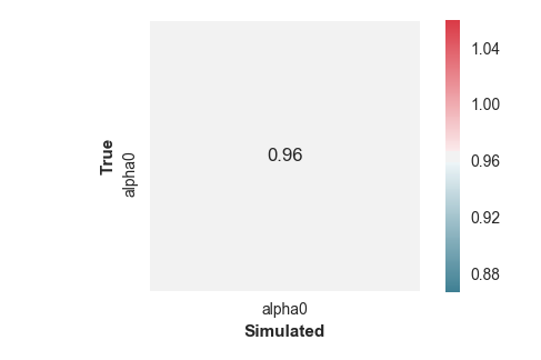
Additionally, the fitting method produced two figures: a scatter plot showing the relationship between the true and estimated alpha values, and a correlation matrix showing the correlation between every estimated parameter in the model (in this case there is only a single value so it’s a pretty uninteresting matrix).
To illustrate this more clearly, let’s look at an example of a more complex model for which parameters aren’t recovered so accurately…
>>> model_1lr.fit_MAP(outcomes, complex_model)
Finished model fitting in 61.4955701763 seconds
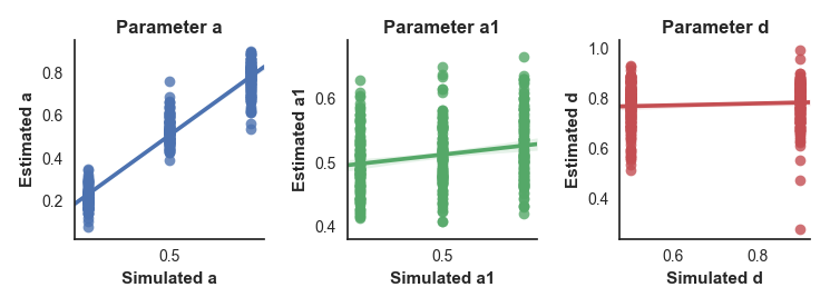
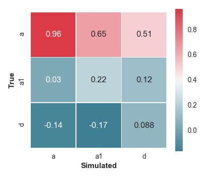
We can see from the plots that it doesn’t look good. The a parameter is estimated successfully, as shown by the scatter plot and a correlation of .96 between the true and estimated values in the correlation matrix. However, the other two parameters show poor correlations between true and estimated values, indicating that we’re not able to recover them successfully.
However, the correlation between simulated and estimated parameters is not always the most appropriate way to judge recovery success, as it is not affected by any bias in the estimated parameter values. For this reason, the correlation plot also provides a line of equality (the dashed black line on the plots) and indicates the R2 value.
Parameter recovery tests can be re-run at any time after fitting a model to simulated data by calling the recovery() method of the model instance.
Simulating noisy data
Real data is often contaminated by some degree of noise, and it can be helpful to produce simulations that reflect this. For this purpose, the simulate method is able to add gaussian-distributed noise to the simulated data. This will be added to the simulated value or probability output, and is enabled by setting the noise argument to True. Two other arguments control the distribution of this noise; the noise_mean argument can be used to change the mean of the distribution, while the noise_sd sets the standard deviation of the distribution. Changing the mean will add a degree of bias to the estimated values, while increasing the standard deviation will make the values more variable. Note that the simulated values will not go above or below the maximum or minmum values provided in the outcomes (i.e. if the maximum outcome value is 1, even with high-variance aded noise the simulated probability estimate will not be higher than 1).
Simulating data from real parameter estimates
We often wish to produce simulated data from the parameter values estimated from fitting the model to real subjects’ data. This can be done by simply calling the simulate() method of a model after fitting has been performed without providing any values for the learning model or observation model parameters. DMpy will use the estimated value for each subject and simulate data from these values. Additionally, if the plot_against_true argument is set to True, a plot will be produced showing the simulated data for each subject along with their true data for comparison.
Technical stuff
Mostly here to help me remember how things work
Inputs to the core functions (get_value and define_simulation_function) expect outcomes/responses/dynamic inputs to to have the shape n_trials X n_columns X n_subjects, where n_columns is the 2nd dimension of the input (e.g. if you have a four arm bandit, this might have four dimensions.
Static parameters are expected to have the shape n_columns X n_subjects.